Mathematics of Diffusion models

Introduction

This blog post aims to develop and explain the mathematical foundations of diffusion models ¹, and image-to-image diffusion models ^{2 3}. This work is part of a larger project on image colorization using diffusion, which was done in collaboration with Brennan Whitfield, and Vivek Shome in 2022. This blog post is inspired by Lilian Weng’s blog post on diffusion models ⁴, but contains more details in the mathematical derivations, which may help in understanding certain aspects.

If you find any mistakes, reasoning problems or other, do not hesitate to contact me, I would be happy to improve this work with your help.

General Idea

The idea of diffusion models is to slowly destroy structure in a data distribution through an iterative forward process. Then, we learn a reverse diffusion process using an neural network, that restores structure in data. This model yield to a highly flexible generative model of the data. This can be seen as a Markov chain of diffusion steps, which slowly add random noise to the data, and then learn to reverse the diffusion process in order to construct new desired data samples from the noise.

In the context of image-to-image diffusion, we use a conditional diffusion model which, on top of requiring a noisy image and timestep, takes an additional image as input.

Notation

The following notation will be adopted for the next parts:

• $\mathcal{N}(x;\mu,\sigma^2)$ : sampling x from a normal distribution of mean $\mu$ and variance $\sigma^2$
• $\mathbf{x_t}$ is the image after applying $t$ iterations of noise through the forward process
• $\mathbf{x_0}$ is the original image, before going through the forward process
• $\mathbf{z}$ is the image which conditions the model (source image we seek to colorize in the context of image colorization)
• $\mathbf{x_T}$ is the final image of the forward process which follows an isotropic Gaussian distribution ($T$ is constant)
• $q(\mathbf{x_t}|\mathbf{x_{t-1}})$ corresponds to the forward process, taking an image $\mathbf{x_{t-1}}$ as input, and output $\mathbf{x_t}$ which contains more noise
• $p_\theta(\mathbf{x_{t-1}}|\mathbf{x_t})$ corresponds to the reverse process, taking an image $\mathbf{x_t}$ as input, and output $\mathbf{x_{t-1}}$ which contains less noise

The Forward Diffusion Process

Let’s sample an image from a real conditional data distribution $\mathbf{x_0} \sim q(\mathbf{x}|\mathbf{z})$. We define a forward diffusion process, in which a small amount of Gaussian noise is iteratively added to the image $\mathbf{x_0}$, in $T$ steps, leading to the sequence of noisy images $\mathbf{x_1},\dots,\mathbf{x_T}$. The step size is controlled by a variance schedule $\beta_t$ going from a start value to an end value defined accordingly to the scale of the pixel’s values, in $T$ steps, starting at $t=1$. The noise added is sampled from a Gaussian distribution. Thus we can define: $$q(\mathbf{x_t}|\mathbf{x_{t-1}}) = \mathcal{N}(\mathbf{x_t};\sqrt{1-\beta_t}\mathbf{x_{t-1}},\beta_t\mathbf{I})$$ Where the variance schedule scales the mean and the variance of the noise sampled from the normal distribution. Since our forward process is a Markov Chain (satisfying Markov property ⁵), we can also write:

\begin{align*} q(\mathbf{x_{1:T}}|\mathbf{x_0}) &= q(\mathbf{x_1}, \dots, \mathbf{x_T} | \mathbf{x_0}) \\
&= \frac{q(\mathbf{x_0}, \mathbf{x_1}, \dots, \mathbf{x_T})}{q(\mathbf{x_0})} &&\text{(Bayes' Theorem)}\\
&= \frac{q(\mathbf{x_0})q(\mathbf{x_1}|\mathbf{x_0})\dots q(\mathbf{x_T}|\mathbf{x_{T-1}})}{q(\mathbf{x_0})} &&\text{(Markov property)}\\
&= q(\mathbf{x_1}|\mathbf{x_0})\dots q(\mathbf{x_T}|\mathbf{x_{T-1}})\\
&= \prod^T_{t=1}q(\mathbf{x_t}|\mathbf{x_{t-1}}) \end{align*}

Additionally, we can improve the forward process further, allowing us to sample a noisy image $\mathbf{x_t}$ at any particular time $t$. First, we let $\alpha_{t} = 1 - \beta_t$, and we also define $\bar{\alpha_t} = \prod\nolimits_{i=1}^t \alpha_i$. Now, we rewrite:

$$q(\mathbf{x_t}|\mathbf{x_{t-1}}) = \mathcal{N}(\mathbf{x_t};\sqrt{\alpha_t}\mathbf{x_{t-1}},(1 - \alpha_t)\mathbf{I})$$

using the reparameterization trick for Gaussian distribution $\mathcal{N}(\mathbf{x}; \mathbf{\mu},\sigma^2\mathbf{I})$,$\mathbf{x} = \mathbf{\mu} + \sigma\mathbf{\epsilon}$, where $\mathbf{\epsilon} \sim \mathcal{N}(\boldsymbol{0}, \mathbf{I})$. This gives us:

\begin{align*} \mathbf{x_t} &= \sqrt{\alpha_t} \mathbf{x_{t-1}} + \sqrt{1-\alpha_t}\mathbf{\epsilon_{t-1}} \\
\mathbf{x_{t-1}} &= \sqrt{\alpha_{t-1}} \mathbf{x_{t-2}} + \sqrt{1-\alpha_{t-1}}\mathbf{\epsilon_{t-2}} && \text{(Repeat for $\mathbf{x_{t-1})}$)} \end{align*}

Now, we combine the above equations:

\begin{align*} \mathbf{x_t} &= \sqrt{\alpha_t} \mathbf{x_{t-1}} + \sqrt{1-\alpha_t}\mathbf{\epsilon_{t-1}} \\
&= \sqrt{\alpha_t} (\sqrt{\alpha_{t-1}} \mathbf{x_{t-2}} + \sqrt{1-\alpha_{t-1}}\mathbf{\epsilon_{t-2}}) + \sqrt{1-\alpha_t}\mathbf{\epsilon_{t-1}} \\
&= \sqrt{\alpha_t \alpha_{t-1}} \mathbf{x_{t-2}} + \sqrt{\alpha_t(1-\alpha_{t-1})}\mathbf{\epsilon_{t-2}} + \sqrt{1-\alpha_t}\mathbf{\epsilon_{t-1}} \end{align*}

Note that we can reverse the reparameterization trick separately on $\sqrt{\alpha_t(1-\alpha_{t-1})}\mathbf{\epsilon_{t-2}}$ and $\sqrt{1-\alpha_t}\mathbf{\epsilon_{t-1}}$, considering them to be samples from $\mathcal{N}(\mathbf{0},\alpha_t(1-\alpha_{t-1})\mathbf{I})$ and from $\mathcal{N}(\mathbf{0},(1-\alpha_t)\mathbf{I})$ respectively. Thus, we can combine these Gaussian distributions with different variance as $\mathcal{N}(\mathbf{0}, ((1-\alpha_t) + \alpha_t(1-\alpha_{t-1}))\mathbf{I}) = \mathcal{N}(\mathbf{0}, (1-\alpha_{t} \alpha_{t-1})\mathbf{I})$. Once again reparameterizing this new distribution:

\begin{align*} \mathbf{x_t} &= \sqrt{\alpha_t \alpha_{t-1}} \mathbf{x_{t-2}} + \sqrt{1-\alpha_{t} \alpha_{t-1}}\mathbf{\epsilon} && \mathbf{\epsilon} \sim \mathcal{N}(\mathbf{0},\mathbf{I}) \end{align*}

This process can be continued all the way to $\mathbf{x_0}$ resulting in:

\begin{align*} \mathbf{x_t} &= \sqrt{\alpha_t \alpha_{t-1}} \mathbf{x_{t-2}} + \sqrt{1-\alpha_{t} \alpha_{t-1}}\mathbf{\epsilon} \\
&\vdots \\
\mathbf{x_t} &= \sqrt{\alpha_t \alpha_{t-1} \dots \alpha_{1}}\mathbf{x_0} + \sqrt{1-\alpha_t \alpha_{t-1} \dots \alpha_{1}}\mathbf{\epsilon} \\
&= \sqrt{\bar{\alpha_t}}\mathbf{x_0} + \sqrt{1 - \bar{\alpha_t}}\mathbf{\epsilon} \end{align*}

Since $\mathbf{x_t} = \sqrt{\bar{\alpha_t}}\mathbf{x_0} + \sqrt{1 - \bar{\alpha_t}}\mathbf{\epsilon}$, we can once more reverse the reparamaterization process to achieve:

$$q(\mathbf{x_t} | \mathbf{x_0}) = \mathcal{N}(\mathbf{x_t};\sqrt{\bar{\alpha_t}}\mathbf{x_0}, (1 - \bar{\alpha_t})\mathbf{I})$$

It is clear that we can quickly sample a noisy image $\mathbf{x_t}$ at any timestep t. Given that we are using a conditional diffusion model, this allows us to randomly sample a timestep during training and quickly compute values as to speed up the process.

The Reverse Process

To reverse the above noising process (i.e. $q(\mathbf{x_{t-1}}|\mathbf{x_t})$ ), we would need to know the entire dataset of possible noised images, which is essentially impossible. Thus, we seek to learn an _approximation_ of this reverse process. We will call this approximation $p_\theta$. Note that since we are using a conditional diffusion model, we make use of our $\mathbf{z}$ from above to condition the reverse process.

As we are describing the same distribution in the forward process, but in the opposite direction, we can use the same Markovian property to write:

\begin{align*} p_{\theta}(\mathbf{x_{0:T}}|\mathbf{z}) &= p_{\theta}(\mathbf{x_{T}}, \dots, \mathbf{x_{0}}|\mathbf{z})\\
&= p(\mathbf{x_{T}}) p_{\theta}(\mathbf{x_{T-1}} | \mathbf{x_{T}},\mathbf{z}) \dots p_{\theta}(\mathbf{x_0} | \mathbf{x_1},\mathbf{z}) && \text{(Markov Property)} \\
&= p_{\theta}(\mathbf{x_T})\prod_{t=1}^{T} p_{\theta}(\mathbf{x_{t-1}} | \mathbf{x_t},\mathbf{z}) \\
\end{align*}

Also, we make mention here that conditioning our $\mathbf{\mu_{\theta}}(\mathbf{x_t}, \mathbf{z}, t)$ on $\mathbf{x_0}$ in:

$$p_{\theta}(\mathbf{x_{t-1}} | \mathbf{x_t}, \mathbf{z}) = \mathcal{N}(\mathbf{x_{t-1}}; \mathbf{\mu_{\theta}}(\mathbf{x_t},\mathbf{z}, t), \beta_t \mathbf{I})$$

,allows us to work with the reverse probabilities far more easily, as conditioning on $\mathbf{x_0}$ provides us the ability to treat this distribution as the forward process ($\mathbf{x_0}$ preceeds any $\mathbf{x_t}$, and we have already discussed that $\mathbf{x_t}$ is a noised $\mathbf{x_0}$) ⁶. We will rewrite this as:

$$q(\mathbf{x_{t-1}} | \mathbf{x_t}, \mathbf{x_0}) = \mathcal{N}(\mathbf{x_{t-1}}; \mathbf{\tilde{\mu_t}}(\mathbf{x_t}, \mathbf{x_0}), \tilde{\beta_t}\mathbf{I})$$

Here, $\mathbf{\tilde{\mu_t}}$ and $\tilde{\beta_t}$ are the theoretical values of mean and variance. This is because we are using the forward process, wherein we are aware of the mean and variance at each step.

Before proceeding into our discussion on the loss function, we would like to make note of the absense of $\mathbf{z}$. The additional condition on $p_{\theta}$ has no (noticeable) mathematical change on the derivation. For the sake of simplicity, we refrain from conditioning on $\mathbf{z}$ in the following section.

Loss Function

Next, we seek to optimize the negative log-likelihood of $p_{\theta}(\mathbf{x_{0}})$, which is the probability of generating images coming from the original data distribution $\mathbf{x_0} \sim q(\mathbf{x} | \mathbf{z})$. We are, in essence, using a Variational Auto Encoder, wherein we want our ‘probabilistic decoder’ $p_{\theta}(\mathbf{x_{t-1}} | \mathbf{x_{t}})$ to closely approximate our ‘probabilistic encoder’ $q(\mathbf{x_{t-1}} | \mathbf{x_{t}})$ ⁷. To accomplish this, we need the ability to compare these two distributions. Thus, we use Kullback-Leibler (KL) divergence to achieve this comparison. The more the distributions are equivalent, the closer the KL divergence is to 0. It follows then that we want to minimize our KL divergence. However, we also should maximize the likelihood that we generate real samples, or $p_{\theta}(\mathbf{x_0})$. Conviently, we can employ Variational Lower Bounds (VLB)/Evidence Lower Bounds (ELBO) to achieve this concurrently ⁸, ⁹. We will refer to Variational Lower Bounds as VLB for the remainder of this article. Since we want to minimize the dissimilarities between the distributions when traversing consecutive steps, we similarly want to minimize the difference between all of the steps ($\mathbf{x_{1:T}}$) which are noised samples, given the initial sample $\mathbf{x_0}$. Thus, we can write this KL divergence as $D_{\text{KL}}(q(\mathbf{x_{1:T}} | \mathbf{x_{0}}) || p_{\theta}(\mathbf{x_{1:T}} | \mathbf{x_{0}}))$.

To derive the VLB, we expand the above KL divergence:

\begin{align*} D_{\text{KL}}(q(\mathbf{x_{1:T}} | \mathbf{x_{0}}) || p_{\theta}(\mathbf{x_{1:T}} | \mathbf{x_{0}})) &= \mathbb{E}_{\mathbf{x_{1:T}} \sim q(\mathbf{x_{1:T}} | \mathbf{x_{0}})} \log{\Big ( \frac{q(\mathbf{x_{1:T}} | \mathbf{x_{0}})}{p_{\theta}(\mathbf{x_{1:T}} | \mathbf{x_{0}})}\Big )} \\
\end{align*}

\begin{align*} &= \int q(\mathbf{x_{1:T}} | \mathbf{x_{0}}) \log{\Big ( \frac{q(\mathbf{x_{1:T}} | \mathbf{x_{0}})}{p_{\theta}(\mathbf{x_{1:T}} | \mathbf{x_{0}})}\Big )} d\mathbf{x_{1:T}} \\
&= \int q(\mathbf{x_{1:T}} | \mathbf{x_{0}}) \log{\Big ( \frac{q(\mathbf{x_{1:T}} | \mathbf{x_{0}}) p_{\theta}(\mathbf{x_{0}})}{p_{\theta}(\mathbf{x_{1:T}}, \mathbf{x_{0}})}\Big )} d\mathbf{x_{1:T}} && \text{(Bayes' Rule)}\\
&= \int q(\mathbf{x_{1:T}} | \mathbf{x_{0}}) \Big [ \log{p_{\theta}(\mathbf{x_{0}})} + \log{\Big ( \frac{q(\mathbf{x_{1:T}} | \mathbf{x_{0}})}{p_{\theta}(\mathbf{x_{1:T}}, \mathbf{x_{0}})}\Big )} \Big ] d\mathbf{x_{1:T}} \\
&= \log{p_{\theta}(\mathbf{x_{0}})} \int q(\mathbf{x_{1:T}} | \mathbf{x_{0}}) d\mathbf{x_{1:T}} + \int q(\mathbf{x_{1:T}} \vert \mathbf{x_{0}}) \log \Big( \frac{q(\mathbf{x_{1:T}} \vert \mathbf{x_{0}})}{p_{\theta}(\mathbf{x_{1:T}}, \mathbf{x_{0}})}\Big) d\mathbf{x_{1:T}}\\
&= \log{p_{\theta}(\mathbf{x_{0}})} + \int q(\mathbf{x_{1:T}} \vert \mathbf{x_{0}}) \log \Big( \frac{q(\mathbf{x_{1:T}} \vert \mathbf{x_{0}})}{p_{\theta}(\mathbf{x_{1:T}}, \mathbf{x_{0}})}\Big) d\mathbf{x_{1:T}} && \text{$\Big( \int f(x)dx = 1\Big)$}\\
&= \log{p_{\theta}(\mathbf{x_{0}})} + \int q(\mathbf{x_{1:T}} \vert \mathbf{x_{0}}) \log \Big( \frac{q(\mathbf{x_{1:T}} \vert \mathbf{x_{0}})}{p_{\theta}(\mathbf{x_{0}} | \mathbf{x_{1:T}}) p_{\theta}(\mathbf{x_{1:T}})}\Big) d\mathbf{x_{1:T}} && \text{(Bayes' Rule)}\\
&= \log{p_{\theta}(\mathbf{x_{0}})} + \int q(\mathbf{x_{1:T}} \vert \mathbf{x_{0}}) \Big [ \log \Big( \frac{q(\mathbf{x_{1:T}} \vert \mathbf{x_{0}})}{p_{\theta}(\mathbf{x_{1:T}})}\Big) - \log p_{\theta}(\mathbf{x_{0}} | \mathbf{x_{1:T}}) \Big ] d\mathbf{x_{1:T}} \\
&= \log{p_{\theta}(\mathbf{x_{0}})} + \int q(\mathbf{x_{1:T}} \vert \mathbf{x_{0}}) \log \Big( \frac{q(\mathbf{x_{1:T}} \vert \mathbf{x_{0}})}{p_{\theta}(\mathbf{x_{1:T}})}\Big) - q(\mathbf{x_{1:T}} \vert \mathbf{x_{0}})\log p_{\theta}(\mathbf{x_{0}} | \mathbf{x_{1:T}}) d\mathbf{x_{1:T}} \\
&= \log{p_{\theta}(\mathbf{x_{0}})} + \mathbb{E}_ {\mathbf{x_{1:T}} \sim q(\mathbf{x_{1:T}} | \mathbf{x_{0}})} \Big [ \log \Big( \frac{q(\mathbf{x_{1:T}} \vert \mathbf{x_{0}})}{p_{\theta}(\mathbf{x_{1:T}})}\Big) - \log p_{\theta}(\mathbf{x_{0}} | \mathbf{x_{1:T}}) \Big ] \\
&= \log{p_{\theta}(\mathbf{x_{0}})} + \mathbb{E}_ {\mathbf{x_{1:T}} \sim q(\mathbf{x_{1:T}} | \mathbf{x_{0}})} \Big [ \log \Big( \frac{q(\mathbf{x_{1:T}} \vert \mathbf{x_{0}})}{p_{\theta}(\mathbf{x_{1:T}})}\Big) \Big ] - \mathbb{E}_ {\mathbf{x_{1:T}} \sim q(\mathbf{x_{1:T}} | \mathbf{x_{0}})} \Big [ \log p_{\theta}(\mathbf{x_{0}} | \mathbf{x_{1:T}}) \Big ] \\
&= \log{p_{\theta}(\mathbf{x_{0}})} + D_{\text{KL}}(q(\mathbf{x_{1:T}} | \mathbf{x_{0}}) || p_{\theta}(\mathbf{x_{1:T}})) - \mathbb{E}_ {\mathbf{x_{1:T}} \sim q(\mathbf{x_{1:T}} | \mathbf{x_{0}})} \Big [ \log p_{\theta}(\mathbf{x_{0}} | \mathbf{x_{1:T}}) \Big ] \\
\end{align*}

If we rearrange this, we get:

$$ \log{p_{\theta}(\mathbf{x_{0}})} - D_{\text{KL}}(q(\mathbf{x_{1:T}} | \mathbf{x_{0}}) || p_{\theta}(\mathbf{x_{1:T}} | \mathbf{x_{0}})) = \mathbb{E}_ {\mathbf{x_{1:T}} \sim q(\mathbf{x_{1:T}} | \mathbf{x_{0}})} \Big[ \log p_{\theta}(\mathbf{x_{0}} | \mathbf{x_{1:T}}) \Big ] - D_{\text{KL}}(q(\mathbf{x_{1:T}} | \mathbf{x_{0}}) || p_{\theta}(\mathbf{x_{1:T}}))$$

The left hand side of this expression yields the desirable relationship with $\log p_{\theta}(\mathbf{x_{0}})$, and thus is our VLB, which we will call $-L_{\text{VLB}}$. Noting that KL divergence is always non-negative:

$$\log{p_{\theta}(\mathbf{x_{0}})} - D_{\text{KL}}(q(\mathbf{x_{1:T}} | \mathbf{x_{0}}) || p_{\theta}(\mathbf{x_{1:T}} | \mathbf{x_{0}})) \leq \log p_{\theta}(\mathbf{x_{0}})$$

As we seek to maximize the log-likelihood, and acknowledging that all maximizations can be expressed in terms of minimization, we once more rewrite the above expression in terms of said minimization:

$$-\log p_{\theta}(\mathbf{x_{0}}) \leq D_{\text{KL}}(q(\mathbf{x_{1:T}} | \mathbf{x_{0}}) || p_{\theta}(\mathbf{x_{1:T}} | \mathbf{x_{0}})) - \log{p_{\theta}(\mathbf{x_{0}})} $$

We may further simplify this VLB:

\begin{align*} L_{\text{VLB}} &= D_{\text{KL}}(q(\mathbf{x_{1:T}} | \mathbf{x_{0}}) || p_{\theta}(\mathbf{x_{1:T}} | \mathbf{x_{0}})) - \log{p_{\theta}(\mathbf{x_{0}})} \\
&= \mathbb{E}_ {\mathbf{x_{1:T}} \sim q(\mathbf{x_{1:T}} | \mathbf{x_{0}})} \Big[ \log \Big (\frac{q(\mathbf{x_{1:T}} | \mathbf{x_{0}})}{p_{\theta}(\mathbf{x_{1:T}} | \mathbf{x_{0}})} \Big) \Big ] - \log{p_{\theta}(\mathbf{x_{0}})} \\
&= \mathbb{E}_ {\mathbf{x_{1:T}} \sim q(\mathbf{x_{1:T}} | \mathbf{x_{0}})} \Big[ \log \Big (\frac{q(\mathbf{x_{1:T}} | \mathbf{x_{0}})p_{\theta}(\mathbf{x_{0}})}{p_{\theta}(\mathbf{x_{1:T}}, \mathbf{x_{0}})} \Big ) \Big ] - \log{p_{\theta}(\mathbf{x_{0}})} && \text{(Bayes' Rule)}\\
&= \mathbb{E}_ {\mathbf{x_{1:T}} \sim q(\mathbf{x_{1:T}} | \mathbf{x_{0}})} \Big[ \log \Big (\frac{q(\mathbf{x_{1:T}} | \mathbf{x_{0}})}{p_{\theta}(\mathbf{x_{0}}, \mathbf{x_1}, \dots, \mathbf{x_{T}})} \Big ) + \log p_{\theta}(\mathbf{x_{0}}) \Big ] - \log{p_{\theta}(\mathbf{x_{0}})} \\
&= \mathbb{E}_ {\mathbf{x_{1:T}} \sim q(\mathbf{x_{1:T}} | \mathbf{x_{0}})} \Big[ \log \Big ( \frac{q(\mathbf{x_{1:T}} | \mathbf{x_{0}})}{p_{\theta}(\mathbf{x_{0:T}})} \Big) \Big ] + \mathbb{E}_ {\mathbf{x_{1:T}} \sim q(\mathbf{x_{1:T}} | \mathbf{x_{0}})} [ \log p_{\theta}(\mathbf{x_{0}}) ] - \log{p_{\theta}(\mathbf{x_{0}})} \\
&= \mathbb{E}_ {q(\mathbf{x_{1:T}} | \mathbf{x_{0}})} \Big[ \log \Big ( \frac{q(\mathbf{x_{1:T}} | \mathbf{x_{0}})}{p_{\theta}(\mathbf{x_{0:T}})} \big ) \Big ] + \log p_{\theta}(\mathbf{x_{0}}) - \log{p_{\theta}(\mathbf{x_{0}})} \\
&= \mathbb{E}_ {q(\mathbf{x_{0:T}} | \mathbf{x_{0}})} \Big[ \log \Big ( \frac{q(\mathbf{x_{1:T}} | \mathbf{x_{0}})}{p_{\theta}(\mathbf{x_{0:T}})} \Big) \Big ]\\
\end{align*}

However, we cannot compute this simplified VLB, as the denominator would require us to already know the reverse conditionals. Thus, we again rewrite our VLB as:

\begin{align*} L_{\text{VLB}} &= \mathbb{E}_ {q} \Big[ \log \Big ( \frac{q(\mathbf{x_{1:T}} | \mathbf{x_{0}})}{p_{\theta}(\mathbf{x_{0:T}})} \Big) \Big ] \\
&= \mathbb{E}_ {q} \Big[ \log \Big ( \frac{\prod\nolimits^T_{t=1}q(\mathbf{x_t}|\mathbf{x_{t-1}})}{p_{\theta}(\mathbf{x_T})\prod\nolimits_{t=1}^{T} p_{\theta}(\mathbf{x_{t-1}} | \mathbf{x_t})} \Big) \Big ] \\
&= \mathbb{E}_ {q} \Big[ -\log{p_{\theta}(\mathbf{x_T})} + \log \Big ( \frac{\prod\nolimits^T_{t=1}q(\mathbf{x_t}|\mathbf{x_{t-1}})}{\prod\nolimits_{t=1}^{T} p_{\theta}(\mathbf{x_{t-1}} | \mathbf{x_t})} \Big) \Big ] \\
&= \mathbb{E}_ {q} \Big[ -\log{p_{\theta}(\mathbf{x_T})} + \sum\nolimits_{t=1}^{T} \log \Big ( \frac{q(\mathbf{x_t}|\mathbf{x_{t-1}})}{p_{\theta}(\mathbf{x_{t-1}} | \mathbf{x_t})} \Big) \Big ] \\
&= \mathbb{E}_ {q} \Big[ -\log{p_{\theta}(\mathbf{x_T})} + \sum\nolimits_{t=2}^{T} \log \Big ( \frac{q(\mathbf{x_t}|\mathbf{x_{t-1}})}{p_{\theta}(\mathbf{x_{t-1}} | \mathbf{x_t})} \Big) + \log \Big( \frac{q(\mathbf{x_1}|\mathbf{x_{0}})}{p_{\theta}(\mathbf{x_{0}} | \mathbf{x_1})}\Big)\Big ] \\
&= (**) \end{align*}

Now, we use Bayes' Rule to expand $q(\mathbf{x_t}|\mathbf{x_{t-1}})$:

\begin{align*} q(\mathbf{x_t}|\mathbf{x_{t-1}}) &= q(\mathbf{x_t}|\mathbf{x_{t-1}}, \mathbf{x_0}) && \text{($q(\mathbf{x_{t-1}}) = q(\mathbf{x_{t-1}}, \mathbf{x_0})$)} \\
&= \frac{q(\mathbf{x_t},\mathbf{x_{t-1}}, \mathbf{x_0})}{q(\mathbf{x_{t-1}}, \mathbf{x_0})} && \text{(Bayes' Rule)}\\
&= \frac{q(\mathbf{x_{t-1}},\mathbf{x_{t}}, \mathbf{x_0})}{q(\mathbf{x_{t-1}}, \mathbf{x_0})}\\
&= \frac{q(\mathbf{x_{t-1}}| \mathbf{x_{t}}, \mathbf{x_0})q(\mathbf{x_{t}}, \mathbf{x_0})}{q(\mathbf{x_{t-1}}, \mathbf{x_0})} && \text{(Bayes' Rule)}\\
&= \frac{q(\mathbf{x_{t-1}}| \mathbf{x_{t}}, \mathbf{x_0})q(\mathbf{x_{t}}| \mathbf{x_0})q(\mathbf{x_0})}{q(\mathbf{x_{t-1}}| \mathbf{x_0})q(\mathbf{x_0})} && \text{(Bayes' Rule)}\\
&= \frac{q(\mathbf{x_{t-1}}| \mathbf{x_{t}}, \mathbf{x_0})q(\mathbf{x_{t}}| \mathbf{x_0})}{q(\mathbf{x_{t-1}}| \mathbf{x_0})} && \text{(Bayes' Rule)}\\
\end{align*}

Returning to our previous system of equivalences:

\begin{align*} (**) &= \mathbb{E}_ {q} \Big[ -\log{p_{\theta}(\mathbf{x_T})} + \sum\nolimits_{t=2}^{T} \log \Big ( \frac{q(\mathbf{x_{t-1}}| \mathbf{x_{t}}, \mathbf{x_0})}{p_{\theta}(\mathbf{x_{t-1}} | \mathbf{x_t})} \cdot \frac{q(\mathbf{x_{t}}| \mathbf{x_0})}{q(\mathbf{x_{t-1}}| \mathbf{x_0})} \Big) + \log \Big( \frac{q(\mathbf{x_1}|\mathbf{x_{0}})}{p_{\theta}(\mathbf{x_{0}} | \mathbf{x_1})}\Big)\Big ] && \text{(Via the above substitution)}\\
&= \mathbb{E}_ {q} \Big[ -\log{p_{\theta}(\mathbf{x_T})} + \sum\nolimits_{t=2}^{T} \log \Big ( \frac{q(\mathbf{x_{t-1}}| \mathbf{x_{t}}, \mathbf{x_0})}{p_{\theta}(\mathbf{x_{t-1}} | \mathbf{x_t})} \Big) + \sum\nolimits_{t=2}^{T} \log \Big( \frac{q(\mathbf{x_{t}}| \mathbf{x_0})}{q(\mathbf{x_{t-1}}| \mathbf{x_0})} \Big) + \log \Big( \frac{q(\mathbf{x_1}|\mathbf{x_{0}})}{p_{\theta}(\mathbf{x_{0}} | \mathbf{x_1})}\Big)\Big ]\\
&= \mathbb{E}_ {q} \Big[ -\log{p_{\theta}(\mathbf{x_T})} + \sum\nolimits_{t=2}^{T} \log \Big ( \frac{q(\mathbf{x_{t-1}}| \mathbf{x_{t}}, \mathbf{x_0})}{p_{\theta}(\mathbf{x_{t-1}} | \mathbf{x_t})} \Big) + \log \Big( \prod \nolimits_{t=2}^{T} \frac{q(\mathbf{x_{t}}| \mathbf{x_0})}{q(\mathbf{x_{t-1}}| \mathbf{x_0})} \Big) + \log \Big( \frac{q(\mathbf{x_1}|\mathbf{x_{0}})}{p_{\theta}(\mathbf{x_{0}} | \mathbf{x_1})}\Big)\Big ]\\
&= \mathbb{E}_ {q} \Big[ -\log{p_{\theta}(\mathbf{x_T})} + \sum\nolimits_{t=2}^{T} \log \Big ( \frac{q(\mathbf{x_{t-1}}| \mathbf{x_{t}}, \mathbf{x_0})}{p_{\theta}(\mathbf{x_{t-1}} | \mathbf{x_t})} \Big) + \log \Big( \frac{q(\mathbf{x_{2}}| \mathbf{x_0}) \dots q(\mathbf{x_{T}}| \mathbf{x_0})}{q(\mathbf{x_{1}}| \mathbf{x_0}) \cdots q(\mathbf{x_{T-1}}| \mathbf{x_0})} \Big) + \log \Big( \frac{q(\mathbf{x_1}|\mathbf{x_{0}})}{p_{\theta}(\mathbf{x_{0}} | \mathbf{x_1})}\Big)\Big ] && \text{(Telescoping product)}\\
&= \mathbb{E}_ {q} \Big[ -\log{p_{\theta}(\mathbf{x_T})} + \sum\nolimits_{t=2}^{T} \log \Big ( \frac{q(\mathbf{x_{t-1}}| \mathbf{x_{t}}, \mathbf{x_0})}{p_{\theta}(\mathbf{x_{t-1}} | \mathbf{x_t})} \Big) + \log \Big( \frac{q(\mathbf{x_{T}}| \mathbf{x_0})}{q(\mathbf{x_{1}}| \mathbf{x_0})} \Big) + \log \Big( \frac{q(\mathbf{x_1}|\mathbf{x_{0}})}{p_{\theta}(\mathbf{x_{0}} | \mathbf{x_1})}\Big)\Big ]\\
&= \mathbb{E}_ {q} \Big[ -\log{p_{\theta}(\mathbf{x_T})} + \sum\nolimits_{t=2}^{T} \log \Big ( \frac{q(\mathbf{x_{t-1}}| \mathbf{x_{t}}, \mathbf{x_0})}{p_{\theta}(\mathbf{x_{t-1}} | \mathbf{x_t})} \Big) + \log \Big( \frac{q(\mathbf{x_{T}}| \mathbf{x_0})q(\mathbf{x_1}|\mathbf{x_{0}})}{q(\mathbf{x_{1}}| \mathbf{x_0})p_{\theta}(\mathbf{x_{0}} | \mathbf{x_1})} \Big) \Big ]\\
&= \mathbb{E}_ {q} \Big[ -\log{p_{\theta}(\mathbf{x_T})} + \sum\nolimits_{t=2}^{T} \log \Big ( \frac{q(\mathbf{x_{t-1}}| \mathbf{x_{t}}, \mathbf{x_0})}{p_{\theta}(\mathbf{x_{t-1}} | \mathbf{x_t})} \Big) + \log \Big( \frac{q(\mathbf{x_{T}}| \mathbf{x_0})}{p_{\theta}(\mathbf{x_{0}} | \mathbf{x_1})} \Big) \Big ]\\
&= \mathbb{E}_ {q} \Big[ -\log{p_{\theta}(\mathbf{x_T})} + \sum\nolimits_{t=2}^{T} \log \Big ( \frac{q(\mathbf{x_{t-1}}| \mathbf{x_{t}}, \mathbf{x_0})}{p_{\theta}(\mathbf{x_{t-1}} | \mathbf{x_t})} \Big) + \log{q(\mathbf{x_{T}}| \mathbf{x_0})}-\log{p_{\theta}(\mathbf{x_{0}} | \mathbf{x_1})}\Big ]\\
&= \mathbb{E}_ {q} \Big[ \log \Big( \frac{q(\mathbf{x_{T}}| \mathbf{x_0})}{p_{\theta}(\mathbf{x_T})} \Big) + \sum\nolimits_{t=2}^{T} \log \Big ( \frac{q(\mathbf{x_{t-1}}| \mathbf{x_{t}}, \mathbf{x_0})}{p_{\theta}(\mathbf{x_{t-1}} | \mathbf{x_t})} \Big)-\log{p_{\theta}(\mathbf{x_{0}} | \mathbf{x_1})}\Big ]\\
&= \mathbb{E}_ {q} \Big[ \mathbb{E}_ {q} \Big[ \log \Big( \frac{q(\mathbf{x_{T}}| \mathbf{x_0})}{p_{\theta}(\mathbf{x_T})} \Big) \Big] + \sum\nolimits_{t=2}^{T} \mathbb{E}_ {q} \Big[ \log \Big ( \frac{q(\mathbf{x_{t-1}}| \mathbf{x_{t}}, \mathbf{x_0})}{p_{\theta}(\mathbf{x_{t-1}} | \mathbf{x_t})} \Big) \Big ]-\log{p_{\theta}(\mathbf{x_{0}} | \mathbf{x_1})}\Big ]\\
&= \mathbb{E}_ {q} \Big[ D_\text{KL} (q(\mathbf{x_{T}}| \mathbf{x_0}) || p_{\theta}(\mathbf{x_T})) + \sum\nolimits_{t=2}^{T} D_\text{KL} ( q(\mathbf{x_{t-1}}| \mathbf{x_{t}}, \mathbf{x_0})||p_{\theta}(\mathbf{x_{t-1}} | \mathbf{x_t})) -\log{p_{\theta}(\mathbf{x_{0}} | \mathbf{x_1})}\Big ]\\
\end{align*}

Now, to make sense of this VLB, we label the components of the above expression as ‘loss terms’ $L_{i}$ where $i = 1, \dots, T$. We have three distinguishable cases ¹:

\begin{align*} L_T &= D_\text{KL} (q(\mathbf{x_{T}}| \mathbf{x_0}) || p_{\theta}(\mathbf{x_T}))\
L_{t-1} &= D_\text{KL} ( q(\mathbf{x_{t-1}}| \mathbf{x_{t}}, \mathbf{x_0})||p_{\theta}(\mathbf{x_{t-1}} | \mathbf{x_t}))\\
L_0 &= -\log{p_{\theta}(\mathbf{x_{0}} | \mathbf{x_1})} \end{align*}

In the case of $L_T$, we are using a pre-defined ‘noise schedule’ and $q$ has no learning parameters.Thus $L_T$ should be considered constant (Recalling that $p_{\theta}(\mathbf{x_T})$ is generated Gaussian noise as well). For $L_{0}$, we might use an additional decoder to model it, and, for lack of time, we will leave this as a constant $C_0$.

As for $L_{t-1}$, we can easily rearrange the above form to achieve an equivalent result for $L_{t}$, where $1 \leq t \leq T-1$:

$$L_{t} = D_\text{KL} ( q(\mathbf{x_{t}}| \mathbf{x_{t+1}}, \mathbf{x_0})||p_{\theta}(\mathbf{x_{t}} | \mathbf{x_{t+1}}))$$

However, as we seek to optimize our VLB, we will manipulate $L_{t}$ in order to find an optimal/viable cost function. To do this, we want some way to measure the ‘loss’ between our predicted noisy images, and the original noisy images themselves. Thus, we manipulate the above loss component to find a usable comparison between the respective distributions. Starting with $L_{t-1}$:

\begin{align*} L_{t-1} &= D_\text{KL} ( q(\mathbf{x_{t-1}}| \mathbf{x_{t}}, \mathbf{x_0})||p_{\theta}(\mathbf{x_{t-1}} | \mathbf{x_t})) \\
&= \mathbb{E}_ {\mathbf{x_{t-1}} \sim q} \Big[ \log \Big( \frac{q(\mathbf{x_{t-1}}| \mathbf{x_{t}}, \mathbf{x_0})}{p_{\theta}(\mathbf{x_{t-1}} | \mathbf{x_{t}}))} \Big) \Big ] \\
&= \mathbb{E}_ {q} \Big[ \log \Big( \frac{q(\mathbf{x_{t-1}}| \mathbf{x_{t}}, \mathbf{x_0})}{p_{\theta}(\mathbf{x_{t-1}} | \mathbf{x_{t}}))} \Big) \Big ] \\
\end{align*}

Recall from above that:

\begin{align*} q(\mathbf{x_{t-1}} | \mathbf{x_t}, \mathbf{x_0}) &= \mathcal{N}(\mathbf{x_{t-1}}; \mathbf{\tilde{\mu_t}}(\mathbf{x_t}, \mathbf{x_0}), \tilde{\beta_t}\mathbf{I}) \\
p_{\theta}(\mathbf{x_{t-1}} | \mathbf{x_t}) &= \mathcal{N}(\mathbf{x_{t-1}}; \mathbf{\mu_{\theta}}(\mathbf{x_t}, t), \beta_t \mathbf{I}) \\
\end{align*}

This allows us to rewrite the expression as:

$$L_{t-1} = \mathbb{E}_ {q} \Big[ \log (\mathcal{N}(\mathbf{x_{t-1}}; \mathbf{\tilde{\mu_t}}(\mathbf{x_t}, \mathbf{x_0}), \tilde{\beta_t}\mathbf{I})) - \log ( \mathcal{N}(\mathbf{x_{t-1}}; \mathbf{\mu_{\theta}}(\mathbf{x_t}, t), \beta_t \mathbf{I})) \Big ]$$

Moving forward, we make use of the assumption that we have a pre-defined noise scheduler (i.e. $\tilde{\beta_t} = \beta_t$ at any timestep t). Additionally, recall that the probability density function of a Gaussian distribution $\mathcal{N}(x;\mu,\sigma^2)$ is:

$$f(x) = \frac{1}{\sqrt{2\pi \sigma^2}}\exp\Big({-\frac{1}{2}\Big({\frac{x-\mu}{\sigma}}\Big)^2}\Big)$$

Again, we manipulate $L_{t-1}$

\begin{align*} L_{t-1} &= \mathbb{E}_{q} \Big[ \log \Big( \frac{1}{\sqrt{2\pi \tilde{\beta_t}}}\exp\Big({-\frac{1}{2}\Big({\frac{x_{t-1}-\mathbf{\tilde{\mu_t}}}{\sqrt{\tilde{\beta_t}}}}\Big)^2}\Big)\Big) - \log \Big( \frac{1}{\sqrt{2\pi \beta_t}}\exp\Big({-\frac{1}{2}\Big({\frac{x_{t-1}-\mathbf{\mu_\theta}}{\sqrt{\beta_t}}}\Big)^2}\Big)\Big) \Big ] \\
&= \mathbb{E}_{q} \Big[ \log \Big( \frac{1}{\sqrt{2\pi \tilde{\beta_t}}} \Big ) + \log \Big( \exp\Big({-\frac{1}{2}\Big({\frac{x_{t-1}-\mathbf{\tilde{\mu_t}}}{\sqrt{\tilde{\beta_t}}}}\Big)^2}\Big)\Big) - \Big( \log \Big( \frac{1}{\sqrt{2\pi \beta_t}} \Big) + \log \Big(\exp\Big({-\frac{1}{2}\Big({\frac{x_{t-1}-\mathbf{\mu_\theta}}{\sqrt{\beta_t}}}\Big)^2}\Big)\Big) \Big) \Big ] \\
&= \mathbb{E}_ {q} \Big[ \log \Big( \exp\Big({-\frac{1}{2}\Big({\frac{x_{t-1}-\mathbf{\tilde{\mu_t}}}{\sqrt{\tilde{\beta_t}}}}\Big)^2}\Big)\Big) - \log \Big(\exp\Big({-\frac{1}{2}\Big({\frac{x_{t-1}-\mathbf{\mu_\theta}}{\sqrt{\beta_t}}}\Big)^2}\Big)\Big) \Big ] && \text{($\tilde{\beta_t} = \beta_t$)} \\
&= \mathbb{E}_ {q} \Big[ \Big({-\frac{1}{2}\Big({\frac{x_{t-1}-\mathbf{\tilde{\mu_t}}}{\sqrt{\tilde{\beta_t}}}}\Big)^2}\Big)- \Big({-\frac{1}{2}\Big({\frac{x_{t-1}-\mathbf{\mu_\theta}}{\sqrt{\beta_t}}}\Big)^2}\Big) \Big ]\\
&= \mathbb{E}_ {q} \Big[ \Big({-\frac{1}{2}\Big({\frac{x_{t-1}-\mathbf{\tilde{\mu_t}}}{\sqrt{\tilde{\beta_t}}}}\Big)^2}\Big)- \Big({-\frac{1}{2}\Big({\frac{x_{t-1}-\mathbf{\mu_\theta}}{\sqrt{\beta_t}}}\Big)^2}\Big)\Big ]\\
&= \mathbb{E}_{q} \Big[ \Big({-\frac{1}{2}\Big({\frac{(x_{t-1}-\mathbf{\tilde{\mu_t}})^2}{\tilde{\beta_t}}}\Big)}\Big)- \Big({-\frac{1}{2}\Big({\frac{(x_{t-1}-\mathbf{\mu_\theta})^2}{\beta_t}}}\Big)\Big)\Big ]\\
&= \mathbb{E}_{q} \Big[ {-\frac{1}{2\beta_t}\Big({(x_{t-1}-\mathbf{\tilde{\mu_t}})^2}}- (x_{t-1}-\mathbf{\mu_\theta})^2\Big)\Big ] && \text{($\tilde{\beta_t} = \beta_t$)} \\
&= (***) \end{align*}

Using aforementioned reparameterization of $\mathbf{x_{t-1}} \sim q(\mathbf{x_{t-1}} | \mathbf{x_t}, \mathbf{x_0}) = \mathcal{N}(\mathbf{x_{t-1}}; \mathbf{\tilde{\mu_t}}(\mathbf{x_t}, \mathbf{x_0}), \tilde{\beta_t}\mathbf{I})$ where $\mathbf{x_{t-1}} = \mathbf{\tilde{\mu_t}} + \sqrt{\tilde{\beta_t}}\mathbf{\epsilon}$ and $\mathbf{\epsilon} \sim \mathcal{N}(\mathbf{0}, \mathbf{I})$, we expand the difference of squares:

\begin{align*} (x_{t-1}-\mathbf{\tilde{\mu_t}})^2- (x_{t-1}-\mathbf{\mu_\theta})^2 &= ((x_{t-1}-\mathbf{\tilde{\mu_t}})+(x_{t-1}-\mathbf{\mu_\theta}))((x_{t-1}-\mathbf{\tilde{\mu_t}})-(x_{t-1}-\mathbf{\mu_\theta}))\\
&= (2x_{t-1}-\mathbf{\tilde{\mu_t}}-\mathbf{\mu_\theta})(\mathbf{\mu_\theta}-\mathbf{\tilde{\mu_t}})\\
&= (2(\mathbf{\tilde{\mu_t}} + \sqrt{\tilde{\beta_t}}\mathbf{\epsilon})-\mathbf{\tilde{\mu_t}}-\mathbf{\mu_\theta})(\mathbf{\mu_\theta}-\mathbf{\tilde{\mu_t}})\\
&= (2\mathbf{\tilde{\mu_t}} + 2\sqrt{\tilde{\beta_t}}\mathbf{\epsilon}-\mathbf{\tilde{\mu_t}}-\mathbf{\mu_\theta})(\mathbf{\mu_\theta}-\mathbf{\tilde{\mu_t}})\\
&= (2\sqrt{\tilde{\beta_t}}\mathbf{\epsilon}+\mathbf{\tilde{\mu_t}}-\mathbf{\mu_\theta})(\mathbf{\mu_\theta}-\mathbf{\tilde{\mu_t}})\\
&= 2\sqrt{\tilde{\beta_t}}\mathbf{\epsilon}\mathbf{\mu_\theta}-2\sqrt{\tilde{\beta_t}}\mathbf{\epsilon}\mathbf{\tilde{\mu_t}}+\mathbf{\tilde{\mu_t}}\mathbf{\mu_\theta}-\mathbf{\tilde{\mu_t}}\mathbf{\tilde{\mu_t}}-\mathbf{\mu_\theta}\mathbf{\mu_\theta}+\mathbf{\mu_\theta}\mathbf{\tilde{\mu_t}}\\
&= 2\sqrt{\tilde{\beta_t}}\mathbf{\epsilon}\mathbf{\mu_\theta}-2\sqrt{\tilde{\beta_t}}\mathbf{\epsilon}\mathbf{\tilde{\mu_t}}-(\mathbf{\tilde{\mu_t}}^2-2\mathbf{\tilde{\mu_t}}\mathbf{\mu_\theta}+\mathbf{\mu_\theta}^2)\\
&= 2\sqrt{\tilde{\beta_t}}\mathbf{\epsilon}\mathbf{\mu_\theta}-2\sqrt{\tilde{\beta_t}}\mathbf{\epsilon}\mathbf{\tilde{\mu_t}}-(\mathbf{\tilde{\mu_t}}-\mathbf{\mu_\theta})^2\\
&= -\Big( (\mathbf{\tilde{\mu_t}}-\mathbf{\mu_\theta})^2 + 2\sqrt{\tilde{\beta_t}}\mathbf{\epsilon}\mathbf{\tilde{\mu_t}} - 2\sqrt{\tilde{\beta_t}}\mathbf{\epsilon}\mathbf{\mu_\theta} \Big)\\
\end{align*}

Returning to (***):

\begin{align*} (***) &= \mathbb{E}_{q} \Big[ -\frac{1}{2\beta_t}\Big({(x_{t-1}-\mathbf{\tilde{\mu_t}})^2}- (x_{t-1}-\mathbf{\mu_\theta})^2\Big)\Big ]\\
&= \mathbb E_q \Big[ \frac{1}{2\beta_t}\Big( (\mathbf{\tilde{\mu_t}}-\mathbf{\mu_\theta})^2 + 2\sqrt{\tilde{\beta_t}}\mathbf{\epsilon}\mathbf{\tilde{\mu_t}} - 2\sqrt{\tilde{\beta_t}}\mathbf{\epsilon}\mathbf{\mu_\theta} \Big) \Big ] \\
\end{align*}

We notice that the clever reparameterization of $\mathbf{x_t}$ as $\mathbf{x_t}(\mathbf{x_0}, \mathbf{\epsilon}) = \sqrt{\bar{\alpha_t}}\mathbf{x_0} + \sqrt{1 - \bar{\alpha_t}}\mathbf{\epsilon}$, lends us:

\begin{align*} &\mathbb E_{\mathbf{x_0}, \mathbf{\epsilon}} \Big[ \frac{1}{2\beta_t}\Big( (\mathbf{\tilde{\mu_t}}-\mathbf{\mu_\theta})^2 + 2\sqrt{\tilde{\beta_t}}\mathbf{\epsilon}\mathbf{\tilde{\mu_t}} - 2\sqrt{\tilde{\beta_t}}\mathbf{\epsilon}\mathbf{\mu_\theta} \Big) \Big ] \\
&= \mathbb E_{\mathbf{x_0}, \mathbf{\epsilon}} \Big[ \frac{1}{2\beta_t} (\mathbf{\tilde{\mu_t}}-\mathbf{\mu_\theta})^2 \Big] + \mathbb E_{\mathbf{x_0}, \mathbf{\epsilon}} \Big[ \frac{1}{\beta_t}\Big(\sqrt{\tilde{\beta_t}}\mathbf{\epsilon}\mathbf{\tilde{\mu_t}} - \sqrt{\tilde{\beta_t}}\mathbf{\epsilon}\mathbf{\mu_\theta} \Big) \Big ] \\
\end{align*}

Here, recall that $\mathbf{\epsilon} \sim \mathcal{N}(\mathbf{0}, \mathbf{I})$, and so $\mathbb{E}_{\mathbf{x_0}, \mathbf{\epsilon}} [\epsilon] = \mathbf{0}$. On top of this, for independent continuous random variables, $\mathbb{E} [XY] = \mathbb{E}[X]\mathbb{E}[Y]$. So, since $\mathbf{x_0}$ and $\mathbf{\epsilon}$ are independent:

\begin{align} &\mathbb E_{\mathbf{x_0}, \mathbf{\epsilon}} \Big[ \frac{1}{2\beta_t} (\mathbf{\tilde{\mu_t}}-\mathbf{\mu_\theta})^2 \Big] + \mathbb E_{\mathbf{x_0}, \mathbf{\epsilon}} \Big[ \frac{1}{\beta_t}\Big(\sqrt{\tilde{\beta_t}}\mathbf{\epsilon}\mathbf{\tilde{\mu_t}} - \sqrt{\tilde{\beta_t}}\mathbf{\epsilon}\mathbf{\mu_\theta} \Big) \Big ] \\
&= \mathbb E_{\mathbf{x_0}, \mathbf{\epsilon}} \Big[ \frac{1}{2\beta_t} (\mathbf{\tilde{\mu_t}}-\mathbf{\mu_\theta})^2 \Big] + \mathbb E_{\mathbf{x_0}, \mathbf{\epsilon}}[\mathbf{\epsilon}] E_{\mathbf{x_0}, \mathbf{\epsilon}} \Big[ \frac{1}{\beta_t}\Big( \sqrt{\tilde{\beta_t}}\mathbf{\tilde{\mu_t}} - \sqrt{\tilde{\beta_t}}\mathbf{\mu_\theta} \Big) \Big ] \\
&= \mathbb E_{\mathbf{x_0}, \mathbf{\epsilon}} \Big[ \frac{1}{2\beta_t} (\mathbf{\tilde{\mu_t}}-\mathbf{\mu_\theta})^2 \Big]\\
L_{t-1} &= \mathbb E_{\mathbf{x_0}, \mathbf{\epsilon}} \Big[ \frac{1}{2\beta_t}\Big( |\mathbf{\tilde{\mu_t}}(\mathbf{x_t}, \mathbf{x_0})-\mathbf{\mu_{\theta}}(\mathbf{x_t}, t)|^2 \Big) \Big] \end{align}

$$\mathbb E_q \Big[ \frac{1}{2\beta_t}\Big( (\mathbf{\tilde{\mu_t}}-\mathbf{\mu_\theta})^2 \Big) \Big] = \mathbb E_q \Big[ \frac{1}{2\beta_t}\Big( |\mathbf{\tilde{\mu_t}}(\mathbf{x_t}, \mathbf{x_0})-\mathbf{\mu_{\theta}}(\mathbf{x_t}, t)|^2 \Big) \Big]$$

Where $| \cdot |$ denotes the one-norm.

Thus, we can see that we have acquired a desired comparison between the two distributions. However, this gives that we are trying to train $\mathbf{\mu_{\theta}}$ to predict $\mathbf{\tilde{\mu_t}}$, which is intuitively difficult to justify. To find a clearer loss function, we look towards parameterizing our means. Starting with $\mathbf{\tilde{\mu_t}}$:

\begin{align*} q(\mathbf{x_{t-1}} | \mathbf{x_t}, \mathbf{x_0}) &= \frac{q(\mathbf{x_{t-1}}, \mathbf{x_t}, \mathbf{x_0})}{q(\mathbf{x_t}, \mathbf{x_0})} && \text{(Bayes' Rule)} \\
&= \frac{q(\mathbf{x_{t}} | \mathbf{x_{t-1}}, \mathbf{x_0})q(\mathbf{x_{t-1}}, \mathbf{x_0})}{q(\mathbf{x_t}| \mathbf{x_0})q(\mathbf{x_0})} && \text{(Bayes' Rule)} \\
&= \frac{q(\mathbf{x_{t}} | \mathbf{x_{t-1}}, \mathbf{x_0})q(\mathbf{x_{t-1}}| \mathbf{x_0})q(\mathbf{x_0})}{q(\mathbf{x_t}| \mathbf{x_0})q(\mathbf{x_0})} && \text{(Bayes' Rule)} \\
&= \frac{q(\mathbf{x_{t}} | \mathbf{x_{t-1}}, \mathbf{x_0})q(\mathbf{x_{t-1}}| \mathbf{x_0})}{q(\mathbf{x_t}| \mathbf{x_0})} \\
&= (\text{****}) \end{align*}

Recall $q(\mathbf{x_{t}} | \mathbf{x_{t-1}}, \mathbf{x_0}) = q(\mathbf{x_{t}} | \mathbf{x_{t-1}})$. Addressing the above distributions individually:

\begin{align*} q(\mathbf{x_{t}} | \mathbf{x_{t-1}}) &= \mathcal{N}(\mathbf{x_t};\sqrt{\alpha_t}\mathbf{x_{t-1}},(1 - \alpha_t)\mathbf{I})\\
q(\mathbf{x_{t-1}}| \mathbf{x_0}) &= \mathcal{N}(\mathbf{x_{t-1}};\sqrt{\bar{\alpha}_{t-1}}\mathbf{x_0}, (1 - \bar{\alpha}_{t-1})\mathbf{I})\\
q(\mathbf{x_t}| \mathbf{x_0}) &= \mathcal{N}(\mathbf{x_t};\sqrt{\bar{\alpha_t}}\mathbf{x_0}, (1 - \bar{\alpha_t})\mathbf{I})\\
\end{align*}

Again using the probability density function of a Gaussian distribution:

\begin{align*} (\text{****}) &= \frac{\frac{1}{\sqrt{2\pi (1 - \alpha_t)}}\exp\Big({-\frac{1}{2}\Big({\frac{\mathbf{x_{t}}-\sqrt{\alpha_t}\mathbf{x_{t-1}}}{\sqrt{(1 - \alpha_t)}}}\Big)^2}\Big)\frac{1}{\sqrt{2\pi (1 - \bar{\alpha}_t})}\exp\Big({-\frac{1}{2}\Big({\frac{\mathbf{x_{t-1}}-\sqrt{\bar{\alpha}_{t-1}}\mathbf{x_0}}{\sqrt{(1 - \bar{\alpha}_{t-1})}}}\Big)^2}\Big)}{\frac{1}{\sqrt{2\pi (1 - \bar{\alpha}_t})}\exp\Big({-\frac{1}{2}\Big({\frac{\mathbf{x_{t}}-\sqrt{\bar{\alpha_t}}\mathbf{x_0}}{\sqrt{(1 - \bar{\alpha_t})}}}\Big)^2}\Big)}\\
&\propto \exp\Big({-\frac{1}{2}\Big({\frac{\mathbf{x_{t}}-\sqrt{\alpha_t}\mathbf{x_{t-1}}}{\sqrt{\beta_t}}}\Big)^2}\Big)+\Big({-\frac{1}{2}\Big({\frac{\mathbf{x_{t-1}}-\sqrt{\bar{\alpha}_{t-1}}\mathbf{x_0}}{\sqrt{(1 - \bar{\alpha}_{t-1})}}}\Big)^2}\Big)-\Big({-\frac{1}{2}\Big({\frac{\mathbf{x_{t}}-\sqrt{\bar{\alpha_t}}\mathbf{x_0}}{\sqrt{(1 - \bar{\alpha_t})}}}\Big)^2}\Big)\\
&= \exp\Big({-\frac{1}{2}\Big({\frac{(\mathbf{x_{t}}-\sqrt{\alpha_t}\mathbf{x_{t-1}})^2}{\beta_t}}}+{\frac{(\mathbf{x_{t-1}}-\sqrt{\bar{\alpha_{t-1}}}\mathbf{x_0})^2}{(1 - \bar{\alpha}_{t-1})}}-{\frac{(\mathbf{x_{t}}-\sqrt{\bar{\alpha_t}}\mathbf{x_0})^2}{(1 - \bar{\alpha_t})}}\Big)\Big)\\
&= \exp\Big({-\frac{1}{2}\Big({\frac{\mathbf{x_{t}}^2-2\mathbf{x_{t}}\sqrt{\alpha_t}\mathbf{x_{t-1}} + \alpha_t\mathbf{x_{t-1}}^2}{\beta_t}}}+{\frac{\mathbf{x_{t-1}}^2-2\mathbf{x_{t-1}}\sqrt{\bar{\alpha}_{t-1}}\mathbf{x_0} + \bar{\alpha}_{t-1}\mathbf{x_0}^2}{(1 - \bar{\alpha}_{t-1})}}-{\frac{(\mathbf{x_{t}}-\sqrt{\bar{\alpha_t}}\mathbf{x_0})^2}{(1 - \bar{\alpha_t})}}\Big)\Big)\\
&= \exp\Big({-\frac{1}{2}\Big({-\frac{2\mathbf{x_{t}}\sqrt{\alpha_t}\mathbf{x_{t-1}}}{\beta_t} -\frac{2\mathbf{x_{t-1}}\sqrt{\bar{\alpha}_{t-1}}\mathbf{x_0}}{(1 - \bar{\alpha}_{t-1})} + \frac{\alpha_t\mathbf{x_{t-1}}^2}{\beta_t}}}+{\frac{\mathbf{x_{t-1}}^2}{(1 - \bar{\alpha}_{t-1})} + \frac{\bar{\alpha}_{t-1}\mathbf{x_0}^2}{(1 - \bar{\alpha}_{t-1})}}+\frac{\mathbf{x_{t}}^2}{\beta_t}-{\frac{(\mathbf{x_{t}}-\sqrt{\bar{\alpha_t}}\mathbf{x_0})^2}{(1 - \bar{\alpha_t})}}\Big)\Big)\\
&= \exp\Big({-\frac{1}{2}\Big(\frac{\alpha_t\mathbf{x_{t-1}}^2}{\beta_t}}+\frac{\mathbf{x_{t-1}}^2}{(1 - \bar{\alpha}_{t-1})} {-\frac{2\mathbf{x_{t}}\sqrt{\alpha_t}\mathbf{x_{t-1}}}{\beta_t} -\frac{2\mathbf{x_{t-1}}\sqrt{\bar{\alpha}_{t-1}}\mathbf{x_0}}{(1 - \bar{\alpha}_{t-1})} + C(\mathbf{x_t}, \mathbf{x_0})}\Big)\Big)\\
&= \exp\Big({-\frac{1}{2}\Big(\Big(\frac{\alpha_t}{\beta_t}}+\frac{1}{(1 - \bar{\alpha}_{t-1})} \Big)\mathbf{x_{t-1}}^2 {-2\Big(\frac{\mathbf{x_{t}}\sqrt{\alpha_t}}{\beta_t} +\frac{\sqrt{\bar{\alpha}_{t-1}}\mathbf{x_0}}{(1 - \bar{\alpha}_{t-1})} \Big)\mathbf{x_{t-1}} + C(\mathbf{x_t}, \mathbf{x_0})}\Big)\Big)\\
\end{align*}

Here $C(\mathbf{x_t}, \mathbf{x_0})$ is function which does not involve $\mathbf{x_{t-1}}$. The reason we choose not to deal with this function involves, again, the probability density function of a normal distribution:

\begin{align*} f(x) &= \frac{1}{\sqrt{2\pi \sigma^2}}\exp\Big({-\frac{1}{2}\Big({\frac{x-\mu}{\sigma}}\Big)^2}\Big) \\
&\propto \exp\Big({-\frac{1}{2}\Big({\frac{x-\mu}{\sigma}}\Big)^2}\Big) \\
&= \exp\Big({-\frac{1}{2}\Big({\frac{x^2-2\mu x + \mu^2}{\sigma^2}}\Big)}\Big) \\
&= \exp\Big({-\frac{1}{2}\Big({\frac{1}{\sigma^2}x^2-\frac{2\mu}{\sigma^2}x + \frac{\mu^2}{\sigma^2}}\Big)}\Big) \\
\end{align*}

Where $\frac{\mu^2}{\sigma^2}$ does not involve $x$.

To continue, we can use the fact that two polynomials are equals if their coefficients are equal. Returning to the above expression, we can correspond $\Big(\frac{\alpha_t}{\beta_t}+\frac{1}{(1 - \bar{\alpha}_{t-1})} \Big)\mathbf{x_{t-1}}^2$ to $\frac{1}{\sigma^2}x^2$. Similarly, $2\Big(\frac{\mathbf{x_{t}}\sqrt{\alpha_t}}{\beta_t} +\frac{\sqrt{\bar{\alpha}_{t-1}}\mathbf{x_0}}{(1 - \bar{\alpha}_{t-1})} \Big)\mathbf{x_{t-1}}$ corresponds to $\frac{2\mu}{\sigma^2}x$. With this information, we parameterize $\tilde{\mu}_{t}(\mathbf{x_t}, \mathbf{x_0})$:

\begin{align*} \tilde{\beta}_{t} &= \Big(\frac{\alpha_t}{\beta_t}+\frac{1}{(1 - \bar{\alpha}_{t-1})} \Big)^{-1} \\
&= \Big(\frac{\alpha_t(1 - \bar{\alpha}_{t-1})+\beta_t}{\beta_t(1 - \bar{\alpha}_{t-1})} \Big)^{-1} \\
&= \frac{\beta_t(1 - \bar{\alpha}_{t-1})}{\alpha_t(1 - \bar{\alpha}_{t-1})+\beta_t} \\
&= \frac{\beta_t(1 - \bar{\alpha}_{t-1})}{\alpha_t - \alpha_t\bar{\alpha}_{t-1}+(1-\alpha_t)} && \text{($\beta_t = 1 - \alpha_t$)}\\
&= \frac{\beta_t(1 - \bar{\alpha}_{t-1})}{1- \bar{\alpha}_{t}} && \text{($\bar{\alpha_t} = \prod\nolimits_{i=1}^t \alpha_i = \alpha_t\bar{\alpha}_{t-1}$)}\\
\end{align*}

\begin{align*} \tilde{\mu}_{t}(\mathbf{x_t}, \mathbf{x_0}) &= \Big(\frac{\mathbf{x_{t}}\sqrt{\alpha_t}}{\beta_t} +\frac{\sqrt{\bar{\alpha}_{t-1}}\mathbf{x_0}}{(1 - \bar{\alpha}_{t-1})} \Big) \Big( \frac{\beta_t(1 - \bar{\alpha}_{t-1})}{1- \bar{\alpha}_{t}} \Big) \\
&= \frac{\mathbf{x_{t}}\sqrt{\alpha_t}}{\beta_t}\Big( \frac{\beta_t(1 - \bar{\alpha}_{t-1})}{1- \bar{\alpha}_{t}} \Big)+\frac{\sqrt{\bar{\alpha}_{t-1}}\mathbf{x_0}}{(1 - \bar{\alpha}_{t-1})}\Big( \frac{\beta_t(1 - \bar{\alpha}_{t-1})}{1- \bar{\alpha}_{t}} \Big) \\
&= \mathbf{x_{t}}\Big( \frac{\sqrt{\alpha_t}\beta_t(1 - \bar{\alpha}_{t-1})}{\beta_t(1- \bar{\alpha}_{t})}\Big)+\mathbf{x_0}\Big( \frac{\sqrt{\bar{\alpha}_{t-1}}\beta_t(1 - \bar{\alpha}_{t-1})}{(1 - \bar{\alpha}_{t-1})(1- \bar{\alpha}_{t})}\Big) \\
&= \mathbf{x_{t}}\Big( \frac{\sqrt{\alpha_t}(1 - \bar{\alpha}_{t-1})}{(1- \bar{\alpha}_{t})}\Big)+\mathbf{x_0}\Big( \frac{\sqrt{\bar{\alpha}_{t-1}}\beta_t}{(1- \bar{\alpha}_{t})}\Big) \\
\end{align*}

We can actually perform a substitution here involving the reparameterization of samples from normal distribution from above: $\mathcal{N}(\mathbf{x}; \mathbf{\mu}, \sigma^2\mathbf{I})$, $\mathbf{x} = \mathbf{\mu} + \sigma\mathbf{\epsilon}$, where $\mathbf{\epsilon} \sim \mathcal{N}(\boldsymbol{0}, \mathbf{I})$.

\begin{align*} q(\mathbf{x_t} | \mathbf{x_0}) &= \mathcal{N}(\mathbf{x_t};\sqrt{\bar{\alpha_t}}\mathbf{x_0}, (1 - \bar{\alpha_t})\mathbf{I}) \\
\mathbf{x_t} &= \sqrt{\bar{\alpha_t}}\mathbf{x_0} + \sqrt{1 - \bar{\alpha_t}}\mathbf{\epsilon_t} \\
\mathbf{x_t} - \sqrt{1 - \bar{\alpha_t}}\mathbf{\epsilon_t} &= \sqrt{\bar{\alpha_t}}\mathbf{x_0}\\
(\sqrt{\bar{\alpha_t}})^{-1}(\mathbf{x_t} - \sqrt{1 - \bar{\alpha_t}}\mathbf{\epsilon_t}) &= \mathbf{x_0}\\
\end{align*}

Returning to $\tilde{\mu}_{t}(\mathbf{x_t}, \mathbf{x_0})$:

\begin{align*} \tilde{\mu}_{t}(\mathbf{x_t}, \mathbf{x_0}) &= \mathbf{x_{t}}\Big( \frac{\sqrt{\alpha_t}(1 - \bar{\alpha}_{t-1})}{(1- \bar{\alpha}_{t})}\Big)+\mathbf{x_0}\Big( \frac{\sqrt{\bar{\alpha}_{t-1}}\beta_t}{(1- \bar{\alpha}_{t})}\Big) \\
&= \mathbf{x_{t}}\Big( \frac{\sqrt{\alpha_t}(1 - \bar{\alpha}_{t-1})}{(1- \bar{\alpha}_{t})}\Big)+(\sqrt{\bar{\alpha_t}})^{-1}(\mathbf{x_t} - \sqrt{1 - \bar{\alpha_t}}\mathbf{\epsilon_t})\Big( \frac{\sqrt{\bar{\alpha}_{t-1}}\beta_t}{(1- \bar{\alpha}_{t})}\Big) \\
&= \frac{\mathbf{x_{t}}\sqrt{\alpha_t}(1 - \bar{\alpha}_{t-1})+(\sqrt{\bar{\alpha_t}})^{-1}(\mathbf{x_t} - \sqrt{1 - \bar{\alpha_t}}\mathbf{\epsilon_t})\sqrt{\bar{\alpha}_{t-1}}\beta_t}{(1- \bar{\alpha}_{t})} \\
&= \frac{\mathbf{x_{t}}\sqrt{\alpha_t}(1 - \bar{\alpha}_{t-1})(\sqrt{\bar{\alpha_t}})+(\mathbf{x_t} - \sqrt{1 - \bar{\alpha_t}}\mathbf{\epsilon_t})\sqrt{\bar{\alpha}_{t-1}}\beta_t}{(\sqrt{\bar{\alpha_t}})(1- \bar{\alpha}_{t})} \\
&= \frac{\mathbf{x_{t}}\sqrt{\alpha_t}\sqrt{\bar{\alpha_t}} - \mathbf{x_{t}}\sqrt{\alpha_t}\sqrt{\bar{\alpha}_{t-1}}\sqrt{\bar{\alpha}_{t-1}}\sqrt{\bar{\alpha_t}}+(\mathbf{x_t} - \sqrt{1 - \bar{\alpha_t}}\mathbf{\epsilon_t})\sqrt{\bar{\alpha}_{t-1}}\beta_t}{(\sqrt{\bar{\alpha_t}})(1- \bar{\alpha}_{t})} && \text{$\bar{\alpha}_{t-1} = \sqrt{\bar{\alpha}_{t-1}}\sqrt{\bar{\alpha}_{t-1}}$}\\
&= \frac{\mathbf{x_{t}}\sqrt{\alpha_t}\sqrt{\alpha_{t}}\sqrt{\bar{\alpha}_{t-1}} - \mathbf{x_{t}}\sqrt{\alpha_t}\sqrt{\bar{\alpha}_{t-1}}\sqrt{\bar{\alpha}_{t-1}}\sqrt{\bar{\alpha_t}}+(\mathbf{x_t} - \sqrt{1 - \bar{\alpha_t}}\mathbf{\epsilon_t})\sqrt{\bar{\alpha}_{t-1}}\beta_t}{(\sqrt{\bar{\alpha}_{t}}\sqrt{\bar{\alpha}_{t-1}})(1- \bar{\alpha}_{t})} && \text{($\alpha_{t} = \alpha_{t}\bar{\alpha}_{t-1}$)}\\
&= \frac{\mathbf{x_{t}}\alpha_t - \mathbf{x_{t}}\sqrt{\bar{\alpha}_{t}}\sqrt{\bar{\alpha_t}}+\mathbf{x_t}\beta_t - \sqrt{1 - \bar{\alpha_t}}\mathbf{\epsilon_t}\beta_t}{\sqrt{\alpha_{t}}(1- \bar{\alpha}_{t})}\\
&= \frac{\mathbf{x_{t}}\alpha_t - \mathbf{x_{t}}\bar{\alpha}_{t}+\mathbf{x_t}\beta_t - \sqrt{1 - \bar{\alpha_t}}\mathbf{\epsilon_t}\beta_t}{\sqrt{\alpha_{t}}(1- \bar{\alpha}_{t})} \\
&= \frac{\mathbf{x_{t}}\alpha_t - \mathbf{x_{t}}\bar{\alpha}_{t}+\mathbf{x_t}(1 - \alpha_t)}{\sqrt{\alpha_{t}}(1- \bar{\alpha}_{t})} - \frac{\mathbf{\epsilon_t}(1 - \alpha_t)}{\sqrt{\alpha_{t}}\sqrt{1 - \bar{\alpha_t}}} && \text{($ \beta_t = 1 - \alpha_t $)} \\
&= \frac{1}{\sqrt{\alpha_{t}}} \Big( \frac{\mathbf{x_{t}}\alpha_t - \mathbf{x_{t}}\bar{\alpha}_{t}+\mathbf{x_t} -\mathbf{x_t} \alpha_t}{1- \bar{\alpha}_{t}} - \frac{1 - \alpha_t}{\sqrt{1 - \bar{\alpha_t}}}\mathbf{\epsilon_t} \Big) \\
&= \frac{1}{\sqrt{\alpha_{t}}} \Big( \frac{\mathbf{x_t} - \mathbf{x_{t}}\bar{\alpha}_{t}}{1- \bar{\alpha}_{t}} - \frac{1 - \alpha_t}{\sqrt{1 - \bar{\alpha_t}}}\mathbf{\epsilon_t} \Big) \\
&= \frac{1}{\sqrt{\alpha_{t}}} \Big( \frac{\mathbf{x_t}(1 - \bar{\alpha}_{t})}{1- \bar{\alpha}_{t}} - \frac{1 - \alpha_t}{\sqrt{1 - \bar{\alpha_t}}}\mathbf{\epsilon_t} \Big) \\
&= \frac{1}{\sqrt{\alpha_{t}}} \Big( \mathbf{x_t} - \frac{1 - \alpha_t}{\sqrt{1 - \bar{\alpha_t}}}\mathbf{\epsilon_t} \Big) \\
\end{align*}

Via a different manipulation of $\mathbf{x_t} = \sqrt{\bar{\alpha_t}}\mathbf{x_0} + \sqrt{1 - \bar{\alpha_t}}\mathbf{\epsilon_t}$, we see we can write $\mathbf{\epsilon}$ parameterized by $\mathbf{x_t}$ and t. Thus, when $\mathbf{\epsilon_{\theta}}(\mathbf{x_t}, t)$, we can perform the above reparameterization to $\mu_{\theta}( \mathbf{x_t}, t)$:

\begin{align*} \mu_{\theta}( \mathbf{x_t}, t) &=\frac{1}{\sqrt{\alpha_{t}}} \Big( \mathbf{x_t} - \frac{1 - \alpha_t}{\sqrt{1 - \bar{\alpha_t}}}\mathbf{\epsilon_{\theta}}(\mathbf{x_t}, t) \Big) \\
\end{align*}

From here, we can return to:

\begin{align*} L_{t-1} &= \mathbb E_{\mathbf{x_0}, \mathbf{\epsilon}} \Big[ \frac{1}{2\beta_t}\Big( |\mathbf{\tilde{\mu_t}}(\mathbf{x_t}, \mathbf{x_0})-\mathbf{\mu_{\theta}}(\mathbf{x_t}, t)|^2 \Big) \Big] \end{align*}

Now, we may rewrite this using our new reparameterizations of $\tilde{\mu}_{t}$ and $\mathbf{\mu_{\theta}}$:

\begin{align*} &= \mathbb E_{\mathbf{x_0}, \mathbf{\epsilon}} \Big[ \frac{1}{2\beta_t}\Big( |\frac{1}{\sqrt{\alpha_{t}}} \Big( \mathbf{x_t} - \frac{1 - \alpha_t}{\sqrt{1 - \bar{\alpha_t}}}\mathbf{\epsilon_t} \Big)-\frac{1}{\sqrt{\alpha_{t}}} \Big( \mathbf{x_t} - \frac{1 - \alpha_t}{\sqrt{1 - \bar{\alpha_t}}}\mathbf{\epsilon_{\theta}}(\mathbf{x_t}, t) \Big)|^2 \Big) \Big] \\
&= \mathbb E_{\mathbf{x_0}, \mathbf{\epsilon}} \Big[ \frac{1}{2\beta_t}\Big( | -\Big(\frac{1 - \alpha_t}{\sqrt{\alpha_{t}}\sqrt{1 - \bar{\alpha_t}}}\mathbf{\epsilon_t} \Big) + \frac{1 - \alpha_t}{\sqrt{\alpha_{t}}\sqrt{1 - \bar{\alpha_t}}}\mathbf{\epsilon_{\theta}}(\mathbf{x_t}, t) |^2 \Big) \Big] \\
&= \mathbb E_{\mathbf{x_0}, \mathbf{\epsilon}} \Big[ \frac{1}{2\beta_t}\Big( | \Big(\frac{1 - \alpha_t}{\sqrt{\alpha_{t}}\sqrt{1 - \bar{\alpha_t}}}\Big) (\mathbf{\epsilon_{\theta}}(\mathbf{x_t}, t)-\mathbf{\epsilon_t})|^2 \Big) \Big] \\
&= \mathbb E_{\mathbf{x_0}, \mathbf{\epsilon}} \Big[ \frac{(1 - \alpha_t)^2}{2\beta_t\alpha_{t}(1 - \bar{\alpha_t})}| \mathbf{\epsilon_t} -(\mathbf{\epsilon_{\theta}}(\mathbf{x_t}, t))|^2 \Big] \\
\end{align*}

As mentioned in other works on this topic, ¹, finds that removing the leading weight term and redefining $L_{t-1}$ as:

$$L_{t-1} := \mathbb E_{\mathbf{x_0}, \mathbf{\epsilon}} \Big[ | \mathbf{\epsilon_t} -(\mathbf{\epsilon_{\theta}}(\mathbf{x_t}, t))|^2 \Big]$$

, yields better performance during training.

Intuitively, we have turned our model $\mathbf{\epsilon}_{\theta}$ into a noise predictor. Essentially, we are training said model (employing a neural network) to closely approximate the level of noise present in an image at a certain timestep $t$, and then substract this noise from the image to reveal a less noised image.

We simplify our entire Loss of $L = L_{0} + L_t + C_t$ down to:

$$L' = L_t + C $$

where $C = L_0 + C_t$ is a constant which do not depends on $\theta$.

Thus, our loss function is complete.

Training and inference algorithms

As mentioned prior to the Loss Function section, we have not conditioned our $p_{\theta}$ on $\mathbf{z}$. This has no effect on the derivation of our loss. However, the algorithms we use during training and inference will differ slightly from a ‘standard’ diffusion model. This is characterized below:

Training algorithm	Inference algorithm

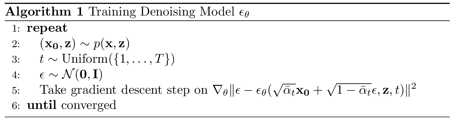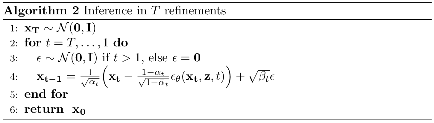$\newline$

The dataset consists of input-output image pairs $\{z_i,x_i\}^N_{i=1}$ where the samples are sampled from an unknown conditional distribution $p(x|z)$. In case of image colorization, $x$ is the color image and $z$ is the grayscale image. This conditional input $z$ is given to the denoising model $\epsilon_\theta$, in addition to the noisy target image $x_t$ and the timestep $t$. In practice, to condition the model we followed the work of ². The input $z$ is concatenated with $x_t$ along the channel dimension before entering the first layer of the neural network.

Citation

Cited as:

Clément, W., Brennan, W., & Vivek, S. (2023). Mathematics of Diffusion Models. https://clement-w.github.io/posts/diffusion

Or

@article{clemw2023diffusion,
  title   = "Mathematics of Diffusion Models",
  author  = "Clément, W. and Brennan, W. and Vivek, S.",
  year    = "2023",
  month   = "Jan",
  url     = "https://clement-w.github.io/posts/diffusion"
}

References

Ho, Jonathan, et al. (2020) “Denoising Diffusion Probabilistic Models” https://arxiv.org/pdf/2006.11239.pdf ↩︎
Saharia, Chitwan, et al. “Image Super-Resolution via Iterative Refinement “. https://arxiv.org/pdf/2104.07636.pdf. ↩︎
Chitwan Saharia, et al. (2022) Palette: Image-to-Image Diffusion Models https://arxiv.org/pdf/2111.05826.pdf ↩︎
Weng, Lilian. (Jul 2021). What are diffusion models? Lil’Log. https://lilianweng.github.io/posts/2021-07-11-diffusion-models/. ↩︎
J. Chang, February 2, 2007. “Markov chains " http://www.stat.yale.edu/~pollard/Courses/251.spring2013/Handouts/Chang-MarkovChains.pdf ↩︎
Jascha Sohl-Dickstein et al. “Deep Unsupervised Learning using Nonequilibrium Thermodynamics.” ICML 2015. https://arxiv.org/abs/1503.03585 ↩︎
Weng, Lilian. 2018. From Autoencoder to Beta-VAE. “https://lilianweng.github.io/posts/2018-08-12-vae/" ↩︎
Feller, W. (1966). An introduction to probability theory and its applications (Vol. 2). John Wiley & Sons. ↩︎
Kingma, Diederik P.; Welling, Max (2014-05-01). “Auto-Encoding Variational Bayes”. https://arxiv.org/abs/1312.6114. ↩︎